一、Pandas

2008年WesMcKinney開發(fā)出的庫

專門用于數(shù)據(jù)挖掘的開源python庫

以Numpy為基礎(chǔ)，借力Numpy模塊在計算方面性能高的優(yōu)勢

基于matplotlib，能夠簡便的畫圖

獨特的數(shù)據(jù)結(jié)構(gòu)

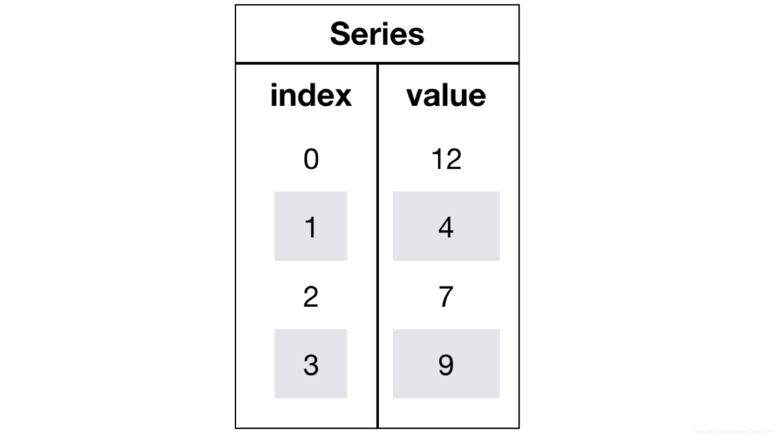
二、數(shù)據(jù)結(jié)構(gòu) Pandas中一共有三種數(shù)據(jù)結(jié)構(gòu)，分別為：Series、DataFrame和MultiIndex。三、Series

Series是一個類似于一維數(shù)組的數(shù)據(jù)結(jié)構(gòu)，它能夠保存任何類型的數(shù)據(jù)，比如整數(shù)、字符串、浮點數(shù)等，主要由一組數(shù)據(jù)和與之相關(guān)的索引兩部分構(gòu)成。

Series的創(chuàng)建

import pandas as pdpd.Series(np.arange(3))

0 01 12 2dtype: int64

#指定索引pd.Series([6.7,5.6,3,10,2], index=[1,2,3,4,5])

1 6.72 5.63 3.04 10.05 2.0dtype: float64

#通過字典數(shù)據(jù)創(chuàng)建color_count = pd.Series({’red’:100, ’blue’:200, ’green’: 500, ’yellow’:1000})color_count

blue 200green 500red 100yellow 1000dtype: int64

Series的屬性

color_count.indexcolor_count.values

也可以使用索引來獲取數(shù)據(jù)：

color_count[2]

100

Series排序

data[‘p_change’].sort_values(ascending=True) # 對值進行排序data[‘p_change’].sort_index() # 對索引進行排序#series排序時，只有一列，不需要參數(shù)

四、DataFrame

創(chuàng)建

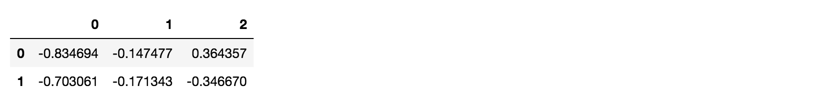
pd.DataFrame(np.random.randn(2,3))

score = np.random.randint(40, 100, (10, 5))score

array([[92, 55, 78, 50, 50],[71, 76, 50, 48, 96],[45, 84, 78, 51, 68],[81, 91, 56, 54, 76],[86, 66, 77, 67, 95],[46, 86, 56, 61, 99],[46, 95, 44, 46, 56],[80, 50, 45, 65, 57],[41, 93, 90, 41, 97],[65, 83, 57, 57, 40]])

但是這樣的數(shù)據(jù)形式很難看到存儲的是什么的樣的數(shù)據(jù)，可讀性比較差！！

# 使用Pandas中的數(shù)據(jù)結(jié)構(gòu)score_df = pd.DataFrame(score)

DataFrame的屬性

data.shapedata.indexdata.columnsdata.valuesdata.Tdata.head(5)data.tail(5)data.reset_index(keys, drop=True)keys : 列索引名成或者列索引名稱的列表drop : boolean, default True.當(dāng)做新的索引，刪除原來的列

dataframe基本數(shù)據(jù)操作

data[‘open’][‘2018-02-27’] # 直接使用行列索引名字的方式（先列后行）data.loc[‘2018-02-27’:‘2018-02-22’, ‘open’] # 使用loc:只能指定行列索引的名字data.iloc[:3, :5 ]# 使用iloc可以通過索引的下標(biāo)去獲取data.sort_values(by=“open”, ascending=True) #單個排序data.sort_values(by=[‘open’, ‘high’]) # 按照多個鍵進行排序data.sort_index() # 對索引進行排序

DataFrame運算

應(yīng)用add等實現(xiàn)數(shù)據(jù)間的加、減法運算應(yīng)用邏輯運算符號實現(xiàn)數(shù)據(jù)的邏輯篩選應(yīng)用isin, query實現(xiàn)數(shù)據(jù)的篩選使用describe完成綜合統(tǒng)計使用max, min, mean, std完成統(tǒng)計計算使用idxmin、idxmax完成最大值最小值的索引使用cumsum等實現(xiàn)累計分析應(yīng)用apply函數(shù)實現(xiàn)數(shù)據(jù)的自定義處理

五、pandas.DataFrame.plot

DataFrame.plot(kind=‘line’)kind : str，需要繪制圖形的種類‘line’ : line plot (default)‘bar’ : vertical bar plot‘barh’ : horizontal bar plot關(guān)于“barh”的解釋：http://pandas.pydata.org/pandas-docs/stable/reference/api/pandas.DataFrame.plot.barh.html‘hist’ : histogram‘pie’ : pie plot‘scatter’ : scatter plot

六、缺失值處理

isnull、notnull判斷是否存在缺失值np.any(pd.isnull(movie)) # 里面如果有一個缺失值,就返回Truenp.all(pd.notnull(movie)) # 里面如果有一個缺失值,就返回Falsedropna刪除np.nan標(biāo)記的缺失值movie.dropna()fillna填充缺失值movie[i].fillna(value=movie[i].mean(), inplace=True)replace替換wis.replace(to_replace='?', value=np.NaN)

七、數(shù)據(jù)離散化

p_change= data[’p_change’]# 自行分組，每組個數(shù)差不多qcut = pd.qcut(p_change, 10)# 計算分到每個組數(shù)據(jù)個數(shù)qcut.value_counts()

# 自己指定分組區(qū)間bins = [-100, -7, -5, -3, 0, 3, 5, 7, 100]p_counts = pd.cut(p_change, bins)

得出one-hot編碼矩陣

dummies = pd.get_dummies(p_counts, prefix='rise')#prefix:分組名字前綴八、數(shù)據(jù)合并

pd.concat([data1, data2], axis=1)按照行或列進行合并,axis=0為列索引，axis=1為行索引

pd.merge(left, right, how=‘inner’, on=None)

可以指定按照兩組數(shù)據(jù)的共同鍵值對合并或者左右各自left: DataFrameright: 另一個DataFrameon: 指定的共同鍵how:按照什么方式連接

九、交叉表與透視表

交叉表：計算一列數(shù)據(jù)對于另外一列數(shù)據(jù)的分組個數(shù) 透視表：指定某一列對另一列的關(guān)系

#通過交叉表找尋兩列數(shù)據(jù)的關(guān)系count = pd.crosstab(data[’week’], data[’posi_neg’])#通過透視表，將整個過程變成更簡單一些data.pivot_table([’posi_neg’], index=’week’)十、數(shù)據(jù)聚合

count = starbucks.groupby([’Country’]).count()col.groupby([’color’])[’price1’].mean()#拋開聚合談分組，無意義

到此這篇關(guān)于Python機器學(xué)習(xí)三大件之二pandas的文章就介紹到這了,更多相關(guān)Python pandas內(nèi)容請搜索好吧啦網(wǎng)以前的文章或繼續(xù)瀏覽下面的相關(guān)文章希望大家以后多多支持好吧啦網(wǎng)！